Multi-resolution voxel-wise neighborhood random forest (MRV-NRF) lesion segmentation

Brian B. Avants, Dorian Pustina, Nicholas J. Tustison

February 22, 2015

Lesion segmentation

Background

We build on the BRATS 2013 challenge to segment areas of the brain that have been damaged by stroke. We also refer to a more recent publication that implements a more complex version of what we do here.

Simulation

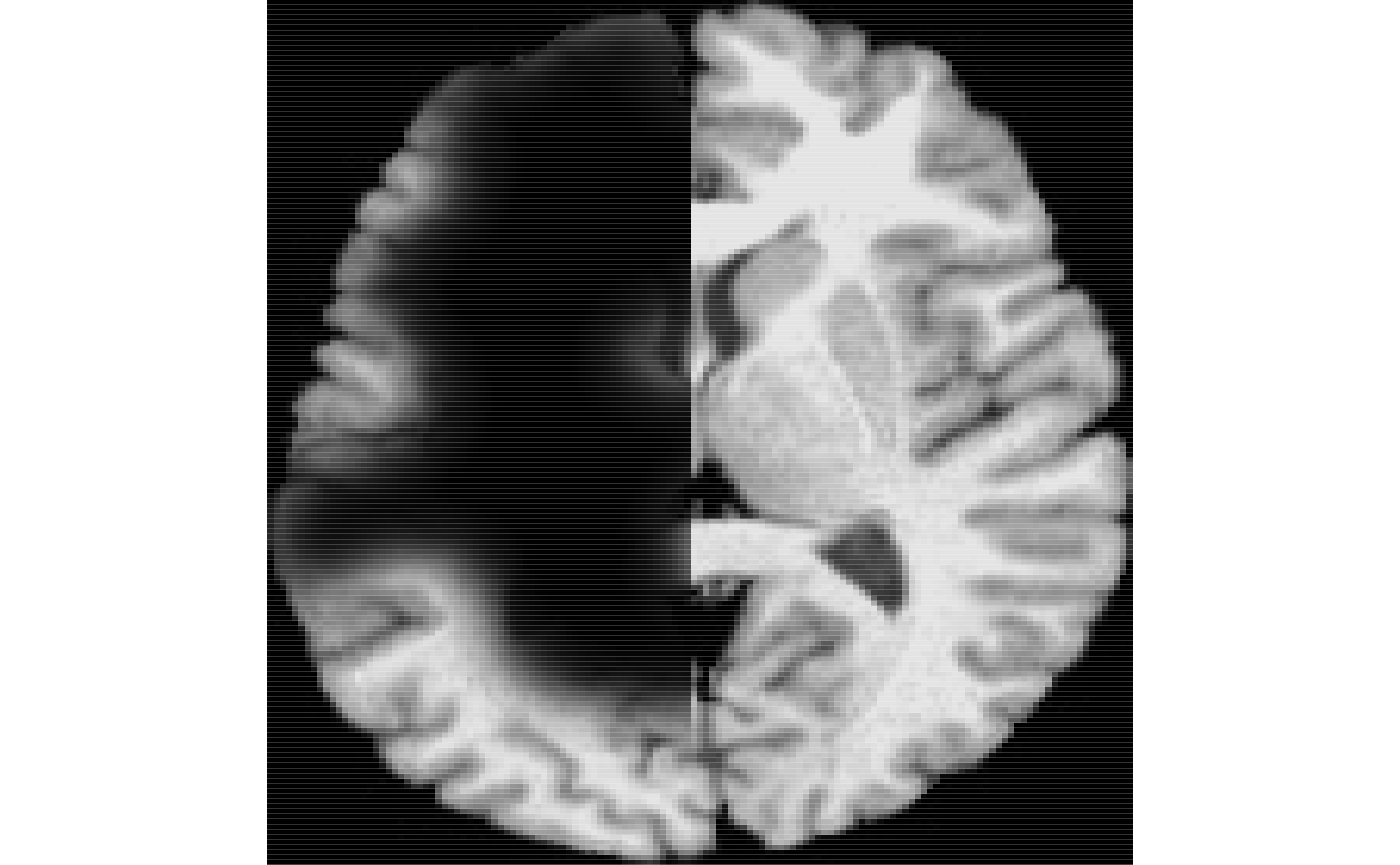
We define a function that will help us simulate large, lateralized lesions on the fly.

library(ANTsR)

## Loading required package: ANTsRCore

## 
## Attaching package: 'ANTsRCore'

## The following objects are masked from 'package:stats':
## 
##     sd, var

## The following objects are masked from 'package:base':
## 
##     all, any, apply, max, min, prod, range, sum

simLesion<-function(  img, s , w, thresh=0.01, mask=NA, myseed )
{
  set.seed(myseed)
  img<-iMath(img,"Normalize")
  if ( is.na(mask) ) mask<-getMask(img)
  i<-makeImage( dim(img) , rnorm( length(as.array(img))  ) )
  i[ mask==0 ]<-0
  ni<-smoothImage(i,s)
  ni[mask==0]<-0
  i<-thresholdImage(ni,thresh,Inf)
  i<-iMath(i,"GetLargestComponent")
  ti<-antsImageClone(i)
  i[i>0]<-ti[i>0]
  i<-smoothImage(i,w)
  i[ mask != 1  ] <- 0
  i[ 1:(dim(img)[1]/2), 1:(dim(img)[2]-1) ]<-0
  limg<-( antsImageClone(img) * (-i)  %>% iMath("Normalize") )
  return( list(limg=limg, lesion=i ) )
}

Generate test data

Now let’s apply this function to generate a test dataset.

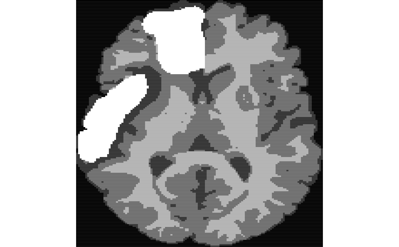
ti<-antsImageRead( getANTsRData("r27") )
timask=getMask(ti)
seg2<-kmeansSegmentation( ti, 3 )$segmentation
ll2<-simLesion( ti, 10, 6, myseed=919 ) # different sized lesion
seg2[ ll2$lesion > 0.5 & seg2 > 0.5 ]<-4

Generate test data

Now let’s apply this function to generate a test dataset.

Make training data

Create training data and map to the test subject. Note that a “real” application of this type would use cost function masking.
But let’s ignore that aspect of the problem here.

Make training data

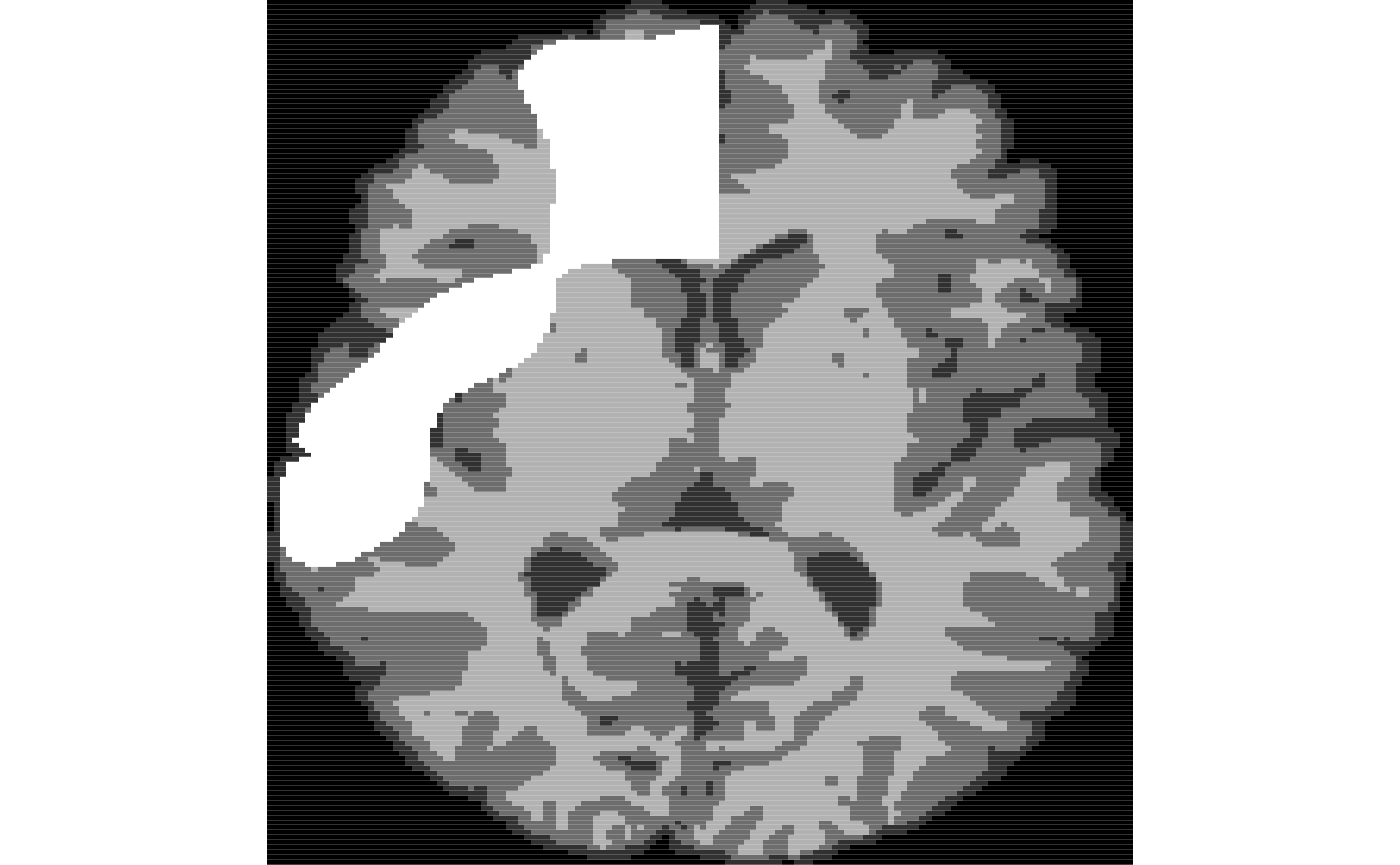
img<-antsImageRead( getANTsRData("r16") )
seg<-kmeansSegmentation( img, 3 )$segmentation
ll<-simLesion( img, 12, 5, myseed=1 )
seg[ ll$lesion > 0.5 & seg > 0.5 ]<-4

Make training data

Pseudo-ground truth

This gives us a subject with a “ground truth” segmentation.

Now we get a new subject and map to the space of the arbitrarily chosen reference space.

Pseudo-ground truth

img<-antsImageRead( getANTsRData("r30") , 2  )
seg1<-kmeansSegmentation( img, 3 )$segmentation
ll1<-simLesion( img, 9, 5,  myseed=2 ) # different sized lesion
seg1[ ll1$lesion > 0.5 & seg1 > 0.5 ]<-4

Pseudo-ground truth

The study

Perform training step

Now use these to train a model.

rad<-c(1,1) # fast setting
mr<-c(1,2,4,2,1) # multi-res schedule, U-style schedule
masks=list(   getMask(seg), getMask(seg1) )
rfm<-mrvnrfs( list(seg,seg1) , list(list(ll$limg), list(ll1$limg) ),
  masks, rad=rad, nsamples = 500, ntrees=1000, multiResSchedule=mr,
  voxchunk=500, do.trace = 100)

## randomForest 4.6-14

## Type rfNews() to see new features/changes/bug fixes.

## ntree      OOB      1      2      3      4
##   100:   8.60% 20.00%  7.49%  9.79%  3.59%
##   200:   8.50% 20.00%  7.49%  9.79%  3.19%
##   300:   9.20% 24.76%  7.82% 10.09%  3.19%
##   400:   9.10% 22.86%  7.82% 10.09%  3.59%
##   500:   9.10% 22.86%  7.82% 10.09%  3.59%
##   600:   9.20% 23.81%  7.82% 10.39%  3.19%
##   700:   9.10% 21.90%  8.14% 10.39%  3.19%
##   800:   9.10% 20.95%  8.47% 10.39%  3.19%
##   900:   9.00% 20.95%  8.14% 10.09%  3.59%
##  1000:   9.00% 20.95%  7.82% 10.39%  3.59%
## ntree      OOB      1      2      3      4
##   100:  11.90% 18.56% 10.27% 16.22%  5.15%
##   200:  12.40% 18.56% 10.88% 16.52%  6.01%
##   300:  11.90% 17.53%  9.67% 16.52%  6.01%
##   400:  11.60% 16.49%  9.37% 16.52%  5.58%
##   500:  11.50% 16.49%  9.67% 15.93%  5.58%
##   600:  11.60% 16.49%  9.97% 15.63%  6.01%
##   700:  11.60% 17.53%  9.67% 15.63%  6.01%
##   800:  11.80% 18.56% 10.27% 15.34%  6.01%
##   900:  11.80% 16.49% 10.57% 15.63%  6.01%
##  1000:  11.90% 16.49%  9.97% 16.22%  6.44%
## ntree      OOB      1      2      3      4
##   100:   6.90%  7.34%  8.25%  9.25%  1.66%
##   200:   6.40%  8.26%  7.30%  8.96%  0.83%
##   300:   6.70%  8.26%  7.62%  9.55%  0.83%
##   400:   6.60%  8.26%  7.30%  9.55%  0.83%
##   500:   6.70%  8.26%  7.62%  9.55%  0.83%
##   600:   6.80%  8.26%  7.30% 10.15%  0.83%
##   700:   6.80%  8.26%  7.30% 10.15%  0.83%
##   800:   6.80%  8.26%  7.30% 10.15%  0.83%
##   900:   6.80%  8.26%  7.30% 10.15%  0.83%
##  1000:   6.80%  8.26%  7.30% 10.15%  0.83%
## ntree      OOB      1      2      3      4
##   100:   7.40% 12.38%  9.12%  8.93%  0.83%
##   200:   6.90% 10.48%  8.81%  8.04%  1.24%
##   300:   7.30% 12.38%  9.12%  8.33%  1.24%
##   400:   7.20% 13.33%  9.43%  7.44%  1.24%
##   500:   7.10% 13.33%  9.12%  7.44%  1.24%
##   600:   7.30% 13.33%  9.75%  7.44%  1.24%
##   700:   7.10% 13.33%  9.43%  7.14%  1.24%
##   800:   7.10% 13.33%  9.12%  7.44%  1.24%
##   900:   7.10% 13.33%  9.12%  7.44%  1.24%
##  1000:   7.20% 13.33%  9.12%  7.74%  1.24%
## ntree      OOB      1      2      3      4
##   100:   6.80% 10.38%  8.62%  8.72%  0.40%
##   200:   7.00%  9.43%  8.92%  9.35%  0.40%
##   300:   6.90%  9.43%  8.92%  9.03%  0.40%
##   400:   6.80%  8.49%  9.54%  8.41%  0.40%
##   500:   7.10%  8.49%  9.85%  9.03%  0.40%
##   600:   6.90%  8.49%  9.54%  8.72%  0.40%
##   700:   6.90%  9.43%  9.23%  8.72%  0.40%
##   800:   7.00%  9.43%  9.54%  8.72%  0.40%
##   900:   7.00%  9.43%  9.54%  8.72%  0.40%
##  1000:   7.00%  9.43%  9.54%  8.72%  0.40%

Combine with additional training runs

newrflist<-list()
temp<-mrvnrfs( list(seg,seg1) , list(list(ll$limg), list(ll1$limg) ),
    masks, rad=rad, nsamples = 500, ntrees=1000, multiResSchedule=mr,
    voxchunk=500 )
for ( k in 1:length( mr ) )
  if ( length( rfm$rflist[[k]]$classes  ) ==
       length( temp$rflist[[k]]$classes )   )
    newrflist[[k]]<-combine( rfm$rflist[[k]], temp$rflist[[k]] )
rfm$rflist<-newrflist

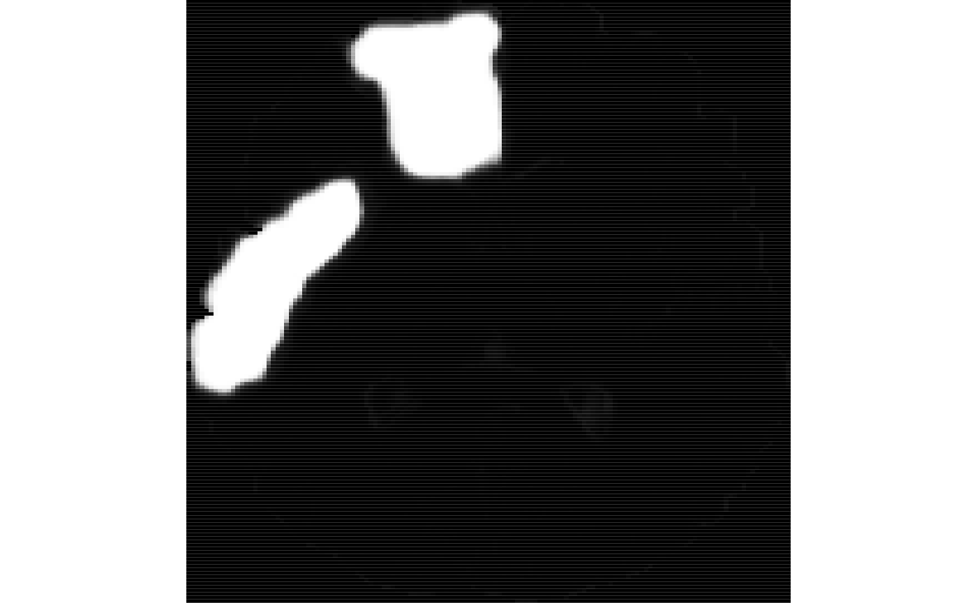
Apply the model to new data

We apply the learned model to segment the new data.

mmseg<-mrvnrfs.predict( rfm$rflist, list(list(ll2$limg)),
  timask, rad=rad, multiResSchedule=mr, voxchunk=500  )

Apply the model to new data

Evaluation

Show ground truth

Here is the ground truth.

Lesion probability

Take a quick look at the lesion probability.

Dice overlap

Now we compute the overlap.

dicenumer<-sum(  mmseg$seg[[1]] == max(mmseg$seg[[1]]) & seg2 == max(seg2) )
dicedenom<-sum( mmseg$seg[[1]] == max(mmseg$seg[[1]]) ) + sum( seg2 == max(seg2)  )
dice <- 2.0 * dicenumer / dicedenom
if ( dice < 0.87 ) stop("suggests performance regression in mrvnrfs")

Summary

The Dice overlap is 0.9099099. We might consider model selection as well where we do a quick estimate of lesion size based on the volume of left hemisphere csf. Then build the model from subjects that “match” with respect to the coarse amount of lesion.